4.1 How To Read a Classical Twin Study
Classical twin studies follow from the logic that regards twins as a “natural experiment”, where observations of a known experience that differs between individuals or over time and is not under the control of the researchers can be used to infer effects of “exposure” to the experience. In the specific case of twin studies, we are drawing conclusions about the effects of sharing 100% versus 50% of your genetic material with a person born at the same time and raised in the same family.
Participants
Monozygotic (MZ, or identical) twins result from the fertilization of a single egg by a single sperm, which then splits creating two zygotes that share 100% of their genetic material. They are naturally occurring genetic clones. Dizygotic (DZ, or fraternal) twins result from the independent fertilization of two eggs by two sperm at the same time. They share on average 50% of their genetic material and are no more or less genetically similar than any pair of full siblings. Conveniently for scientific inference, both types of twins happen to be born at the same time and the overwhelming majority are raised together, so we can ask ourselves: How similar are MZ twins to one another? And are MZ twins more similar to one another than DZ twins are? Because the answer to these questions rests on comparing the correlation between MZ twins (rMZ) to the correlation between DZ twins (rDZ), there need to be enough twin pairs included in the study to estimate a correlation well (more is better; 20 of each type is too few; 100 of each type is probably ok; 200+ of each type and I feel a lot better).
Effect sizes
Most commonly, you will be looking for standardized (that is, sum-to-1.0 or sum-to-100%) estimates of additive genetic (A, or a^2), shared or common environmental (C, or c^2), dominant genetic (D, or d^2), and non-shared or unique environmental (E or e^2) effects. For statistical reasons described below, we are limited to estimating three of those four potential sources of influences on individual differences, or “variance components,” so you will commonly find papers referring to fitting an ACE model or an ADE model. These are the factors they are referring to.
How similar are MZ twins? This question allows us to address the issue of genetic determinism, and to estimate a variance component that behavior geneticists label non-shared or unique environmental influence. We usually describe twin similarity in terms of the correlation (r) between Twin 1’s phenotype and Twin 2’s phenotype. Correlations can be between 0 and 1 and can be either positive or negative. A correlation that is closer to 1 indicates that you would be very accurate at guessing the result of Measure 2 if you knew Measure 1 (or vice versa). A correlation closer to 0 indicates that you wouldn’t do better than random chance at trying to guess Measure 2 from Measure 1 (or vice versa). A positive correlation indicates that as the scores on one measure go up, the scores on the other measure are expected to go up; a negative correlation means that as scores on one measure go up, scores on the other go down. If the only influence on an outcome was genetics, and MZ twins share 100% of the same DNA, then we would expect the MZ twin correlation (rMZ) to be exactly equal to 1. Any rMZ lower than 1 suggests that there are non-genetic influences on the twins’ phenotypes that make them different. They could potentially be anything: different experiences, similar experiences responded to differently by each twin, or just pure measurement error (when we measure something poorly, it cannot correlate highly with other measures). We refer to these difference-making experiential factors as non-shared or unique environmental influences (E), and can estimate them from just rMZ using a Falconer (the guy who derived it) equation of:
(eq. 3.1) E = 1 - rMZ
We might have a problem if rMZ ever went negative (as in, if one twin becoming more something led the other twin to become less of that thing), but practically speaking that doesn’t happen for any of the measures that we use. It’s important to note that to calculate rMZ and estimate E, all we need to measure is the phenotype. We haven’t measured anything specific about E, so we can’t really say for sure what ‘E’ is - we just know that it’s stuff that is unshared or unique between MZ twins, even those raised in the same household.
Are MZ twins more similar than DZ twins? Knowing whether and how much MZ twins are more similar than DZ twins allows us to estimate two other influences on individual differences (or variance components). One is additive genetic influences (A), a second is shared or common environmental influences (C), and a third is dominant genetic influences (D). There are no typos in the preceding sentences; when we only know the MZ twin correlation (rMZ) and the DZ twin correlation (rDZ), we’re going to need to choose whether we estimate C or D, but we can use the twin correlations to guide the choice.
If rMZ is greater than rDZ, that suggests that there is something systematically making MZ twins more similar to one another on the phenotype than DZ twins - but what do MZ twins share more in common than DZ twins? We assume that it is genetics, and Falconer derived a handy estimate of additive genetic influences, which presumes that DZ twins are half as genetically similar as MZ twins, but still more similar than any two random individuals in the population, therefore additive effects could be estimated as twice the difference between their correlations:
(eq. 3.2) A = 2 (rMZ - rDZ)
Note this would cause a problem (that is, a negative A estimate) if the rDZ correlation was larger than the rDZ correlation but, like rMZ being negative, it just doesn’t happen in practice.
Now, we need to decide whether to estimate shared or common environmental effects (C) or dominant genetic effects (D), and because of the limited information we have, we can’t estimate both at the same time. A key assumption here that has gone unstated so far is that the variance for the phenotype, whatever it is, is equal to 1 in both Twin 1 and Twin 2 (correlations are a standardized metric, meaning the measured have been adjusted or standardized to a variance of 1). So we actually have 4 pieces of information: the variance of the phenotype in Twin 1 and Twin 2, the MZ twin correlation, and the DZ twin correlation. In model fitting (even algebraically) you are limited to estimating: the number of pieces of information - 1. The short version is: the math breaks.
So, accepting that without more data (such as correlations among different kinds of family relationships beyond just twins, which absolutely does exist for some datasets but is an added time and money cost that isn’t as widely available as the base just-the-twins participant recruitment approach) we cannot estimate A, C, D, and E simultaneously, and also knowing that A and E are always non-zero (because rMZ > rDZ and rMZ < 1), we are left to choose between C and D, and to do this it helps to define them.
Shared or common environmental influences (C) are (statistically speaking) things that make individuals who share an environment (usually defined as being raised together) more similar to one another, regardless of their genetic similarity. These sorts of influences would be expected to make twins more similar to one another across the board; so C makes rMZ greater than 0, but also make rDZ greater than 0, too, meaning that we would expect the outcome to be that MZ twins and DZ twins are more similarly similar than if that similarity was just down to differences in genetic similarity dosages alone, or, where rMZ < 2*rDZ (that is, when MZ twins are less than twice more similar than DZ twins). C influences can be estimated using the Falconer equation:
(eq. 3.3) C = 2*rDZ - rMZ
Dominant genetic influences (D) are defined as influences that make MZ twins more than twice as similar as DZ twins (so anything that makes them more similar and/or DZ twins less similar than the simple twice-as-much genotype comparison between the two twin types). This could refer to Mendelian-like dominance patterns but, statistically speaking, could arise from ANY non-linear relationship between genetic similarity and phenotype outcome, including gene-environment correlation and gene-environment interaction. D effects are implied when rMZ > 2*rDZ and are relatively rare across all phenotypes with one notable exception: personality. When we examine meta-analyses of twin studies of personality, we reliably find that the broad-sense heritability, or what is often labeled H or h^2 (encompassing both A and D components), is approximately 40%, with no-to-little C, and the rest due to E. But that overall heritability of 40% is about half A, half D (typical twin correlations are around rMZ = 0.45, rDZ = 0.15).
Common tables and figures
When we actually estimate ACE or ADE variance components in a twin study, although it is quite typical to report the raw twin correlations (because BG folks love to estimate Falconer equations in our heads - it’s a fun party trick?), we don’t usually rely on these estimates for the primary conclusions, and they become increasingly unhelpful as more complicated models are attempted, such as examining the relationship between two phenotypes, or the effect of one on another, or change over time.
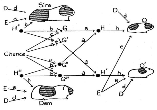
Path diagrams. Structural equation modeling (SEM) or path analysis allows us to derive predictions for the variances and covariances among variables (whether observed or inferred) under a specified model (that is, we have to define the possible relationships that may exist and should be estimated). To do that, we present relationships between variables using diagrams. The relationships can also be represented as structural equations or covariance matrices, but most people would rather have a picture. The first-ever path diagram (below, by Sewell Wright) was all about guinea pig inheritance.

Now we sadly use circles, squares, and triangles in place of guinea pigs, but the interpretation is largely the same. Arrows indicate a directional influence from one thing (at the base of the arrow) to another (at the point). A double-headed arrow indicates a correlation between two things, without implying a particular direction. Concepts that are represented by squares are manifest variables (things that were actually observed or measured; in a twin study, these would be the phenotype measures of Twin 1 and Twin 2). Circles indicate latent variables (things that are not actually observed or measured, but rather are inferred to exist based on the statistical properties of the observed data; in a twin study, A, C, D, and E are latent variables). The number placed along a single- or double-headed arrow (the path estimate or parameter estimate) indicates the strength of the relationship that exists between the two variables. There are some really neat characteristics of path diagrams that allow you to infer the relationship between disparate manifest and/or latent variables by multiplying the parameters along connecting paths. Most importantly, it’s a flexible, universal notation methodology that allows us to change, add, and remove concepts and relationships and still be able to convey our statistical model to a wide audience. So, you’re going to FREQUENTLY encounter path diagrams in the twin study literature.
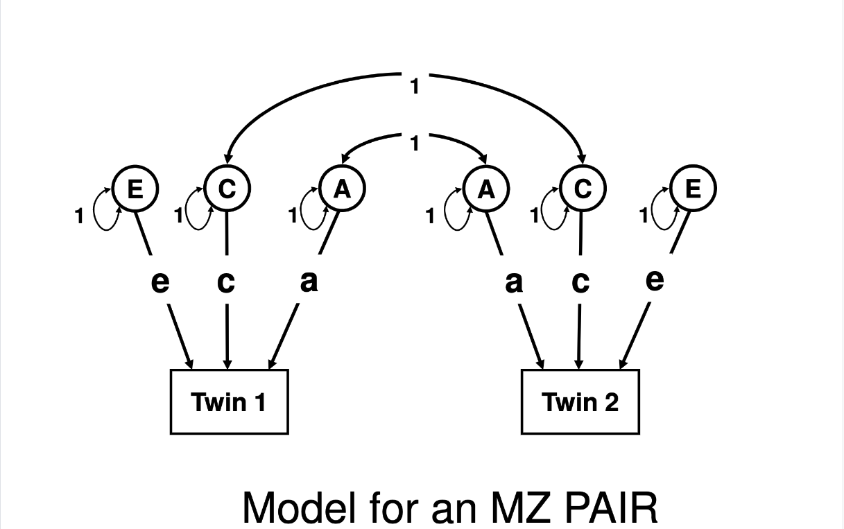
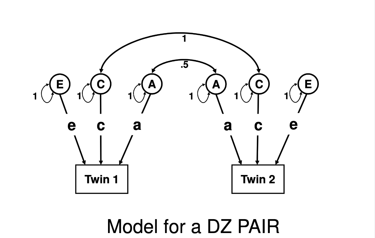
There is exactly one difference between the pictures below, which are the path diagrams describing a standard ACE twin model. It is the entire basis of all of our estimates from classical twin studies.


Did you spot it? The 2nd-to-the top line across the center of the diagram, that indicates the correlation (double-headed arrow) in A (additive genetic) factors between Twin 1 and Twin 2: in the MZ pair model that correlation is “1”, in the DZ pair model that correlation is “0.5”. The C (shared environmental) factors are defined as being correlated at 1 between Twin 1 and Twin 2 regardless of whether they are MZ or DZ pairs, and the E (non-shared environmental) factors are uncorrelated (with no line connecting them, the correlation will be defined as 0 since it is neither included nor estimated. The arrows from the latent factors of A, C, and E to each of the Twins in each model are labeled the same (that is, regardless of MZ or DZ, Twin 1 or Twin 2, they’re labeled “a”, “c”, and “e”) which tells us that when the model is estimated, by definition those parameters (variable/placeholders for numbers to be estimated) will be –by definition– held equal across all individuals (that is, it is the average influence of those factors; you cannot get an individual-specific estimate of genetic/environmental influence from this model).
Note: The difference between the set-up for an ACE model versus the setup for an ADE model is whether the correlation between Twin 1 and Twin 2 “middle” component is 1.0 in both the MZ and DZ models (estimating C, which is shared 100% between twins regardless of zygosity), or 1.0 in the MZ model and 0.25 in the DZ model (which would estimate D, which is shared more than twice as much between MZs than DZs).
Model fit statistics. When these and similar models are estimated, we use a method called Maximum Likelihood Estimation, where a program estimates the most likely values of a population or model parameter value given the observed data. Essentially, it runs through a guess-and-check process: pick some parameter values, see how well they reproduce the observed data, adjust, check again, until further adjustments don’t get any closer to matching the actual data. This is (thankfully) an automated process, so typically 10,000 iterations (or guess-and-check steps) get you a model that is as close as you’ll get to observed reality, given the model that you’ve asked the computer to estimate.
One way we commonly compare alternative models is by looking at model fit statistics. There are a huge variety of ways we can summarize “how well the final model fits the observed data.” Typically model comparisons are made in a table that will have a (hopefully) clear note including what models were compared and how the “best” model was determined (some common measures are AIC and BIC, where smaller numbers are better, and RMSEA, where smaller numbers are also better but for different reasons, and CFI and TLI, where larger numbers are better). But, in the end, it’s the conclusion that matters and these model fit statistics rarely (or debatably) have any absolute interpretation - there’s never going to be a conclusion that suggests they’ve found the True model, just identification of one that was tested better fitting the current data than the others that happen to be tested/testable (again, constrained by information provided by the available data). Alternative models usually try adding or dropping concepts, or fixing or freeing parameters, and see which of many models does the best job reproducing the observed data. Typically, the researchers will identify the best model that was tested on the current data (using whatever metric) and focus on the results of that one model in particular.
Next: 4.2. How To Read a GWAS
Previous: 4.0. Reading Behavior Genetics Research
Home: Table of Contents